May 4, 2025

Gilles Perez • May 04, 2025
Overview of the groundcover eBPF-based APM platform & plans
Q&A about product and any organizational customization needs
30-minute live technical product demo
By submitting this form you agree to our friendly privacy policy.

Monitor everything, deploy in minutes.
Cover your entire Kubernetes stack instantly
with no code changes.
Auto-detect issues across your entire cluster.
See it all. Store what matters. Pay Accordingly.

Discover Caretta, a tool designed for K8s clusters. Generate visual network maps and leverage eBPF for efficient service mapping.

Scientists have long known that the turtles, like many animals, navigate at sea by sensing the invisible lines of the magnetic field, similar to how sailors use latitude and longitude.
But the common sea turtle does much more than that. Turtles also rely on the Earth's magnetic field to find their way home, using the unique magnetic signature of their birth coastline as an internal compass.
Turtles have effectively tamed the wilderness of the open ocean. What can be seen to some animals as an infinite unknown is mapped to the finest of details inside the head of the sea turtle.
From the sea to the cloud, it’s all too easy to get lost in a typical Kubernetes cluster. Gaining a decent understanding of the inter-dependencies between the different workloads running in the cluster is a complicated task, leaving teams to work hard for impactful, actionable insights such as identifying central points of failure or pinpointing security anomalies.
One approach to tackle this issue is visualization: In many ways, a K8s cluster can be seen as a geographic area, with paths and trails forged by communications between different workloads. And just as a map helps familiarize you with your neighborhood and how to navigate around it, it can help you “get around” your K8s cluster.
This is part of the mission of cloud-native observability tools - no APM product is complete without network tracing capabilities of some kind, and data from these traces can help one answer those aforementioned questions. But continuing the approach from our previous post on Murre, what if I only want a minimalistic, efficient solution?
So, what is the easiest way we can map our cluster?
Introducing Caretta - a standalone OSS tool that does just that. Let’s dive into how it works, how it leverages eBPF technology to be lightweight and frictionless, and the obstacles and challenges we encountered on our journey to building it. The end result could be digested directly as raw Prometheus metrics, or you can integrate it into your Grafana with some of our pre-made panels:

First thing we’ll need to figure out is how we get the network data. The naive approach would be using a sniffing tool like tcpdump to gain network observability. But that can be overkill - we don’t need to actually capture the network traffic, we just want to know it exists. As suggested above, we can use eBPF to probe just the data we need.
eBPF who?
If you haven’t already heard of eBPF I can tell you that people like Brendan Gregg call it an "invaluable technology" and compare it to JavaScript:
So instead of a static HTML website, JavaScript lets you define mini programs that run on events like mouse clicks, which are run in a safe virtual machine in the browser. And with eBPF, instead of a fixed kernel, you can now write mini programs that run on events like disk I/O, which are run in a safe virtual machine in the kernel.
eBPF was introduced in early 2014, expanding on BPF's original architecture by providing tools that allow complex programs to run directly in the Linux kernel space.
OK, now you’re probably asking yourself what running the kernel space even means. Basically, it's code running in higher privileges, as opposed to running in "user space" like standard applications. It allows the code to run very efficiently, access low-level kernel resources that would otherwise be complicated and costly (in terms of resource overhead) to access from within user space, but most importantly: it lets you observe any and all programs running in user space – which is hard to do when relying on observability tools that operate in user space themselves.
This is a big thing. It’s basically a new way of equipping the Linux kernel with a programmable, highly efficient virtual machine, allowing programmers access into what was before the sole realm of kernel-developers.
Observability is where eBPF shines. It allows teams to monitor their running applications with a completely out-of-band approach that requires zero code changes or R&D efforts. eBPF enables powerful advantages for observability applications by providing a faster, less resource intensive and holistic approach to gather high precision data.
eBPF offers many ways to capture data from a running system. The kernel allows developers who use eBPF to attach their programs to various types of probes - places in the code of the kernel or applications that when reached, will run the programs attached to them before or after executing their original code. This diagram shows some of the probes available for eBPF:

Working on this project, I was inspired by tcplife - a nifty tool to calculate statistics and information of TCP lifespans, using only a single eBPF probe. The thing is, the kernel already does half of the job for us as it maintains information, such as throughput, for each socket. By probing the tcp_set_state kernel function, tcplife is aware of the active network connection and is accessible to data the kernel maintains for them. Beside having minimal footprint, another advantage of probing specific kernel functions is covering all possible data flows - compared to probing a bunch of possible syscalls the application might use, such as read() or recv(). When application-level context is unnecessary, “sitting” close to the root of the tree lets you cover its branches more easily.
Sounds great - but we’d still be missing something. tcp_set_state is called when, obviously, the state of the TCP connection is being set. For example, when a server starts listening, or when a server-client connection is established, or when a connection is closed. But TCP connections can go long without changing their state, and relying on tcp_set_state will keep us blind to them.
We set out to look for an additional probe that can help us complete the picture. Even then, we find eBPF useful to explore the linux TCP stack. Tools like stacksnoop or stackcount can be used to understand the flow a network packet is going through when it’s processed and compare different functions to see how “noisy” each function is. Searching for data probing locations consists of a constant trade-off between being too nosy and being blind, and we’re looking for the sweet spot in the middle.
In our case, we found the tcp_data_queue function suitable for our needs:
This function is called as one of the final steps of tcp_rcv_established, the function used when receiving packets in the ESTABLISHED state:
So it covers the blindspot of tcp_set_state, and is called only if all previous steps were successful.
Another advantage to using this function is that like tcp_set_state, and most of the kernel TCP functions, its first argument is a struct sock object. This is a big, important kernel struct and we’ll soon dive into the advantages and disadvantages of relying on it to retrieve data, but for now we’ll say it’s convenient that both our probes share a consistent approach to the data.
To recap our collection mechanism - we’ll probe tcp_data_queue to observe the network sockets updating its stats in their established state, and tcp_set_state to track their lifecycle.
As mentioned, our “supply” of data comes from internal kernel network stack objects of a struct called sock. Socks actually wrap other data structures for TCP and INET, so having them means having the data for lower levels of the connection as well. Information like the connection’s 4-tuple (source IP, source port, destination IP and destination port) can be easily retrieved from the sock, especially using the CO-RE approach.
Some issues arise from using kernel internal structures. For example, instead of allocating a new sock each time, the kernel may reuse closed structs. Apparently, socks reusing might occur frequently, and if we do not keep track of socks ending and starting it can lead to collisions and disinformation.
Another difficult issue for extracting the data out of the sock was understanding the role of our host. The sock contains source IP and destination IP, but has no information about who’s the client or the server in this connection. For new socks, we can see (in tcp_set_state) if it goes through TCP_SYN_RECV or TCP_SYN_SENT to understand the side of the equation it’s on; But if the connection was already established, we can’t see the previous states it’s gone through.
The solution we found was examining a field in the sock struct called sk_max_ack_backlog. It holds the maximal length of the accept queue, and is assigned as part of the listen() function of the connection. Which means, that if it is assigned a positive number, the sock went through a listen state, and therefore is a server - and vice versa. That information gives us the direction of the link and the relevant port to store.
So we figured out how to deal with those sock structures. But we’re not really interested in them - we’re interested in it at a higher level. If a client queries a server hundreds of times one after another, we’d like to address it as a single edge in the graph. So the next thing we’re going to do is aggregating what we see in the kernel probes to start counting Links (tuples of client, server and server-port) and their Throughputs. The eBPF program will maintain a map of the sockets it observes, and a userland program accessible to this map will poll over it and generalize each connection to a link and aggregate the throughputs. We’ll run this program on each node in our cluster, and every instance of it will publish the results as metrics to be scraped by a centralized pod.
Let’s talk about the structure of our data. We basically want to have a counter for each link, which is populated by aggregating smaller counters - the ones maintained by the kernel. Sockets can come and go, so we need to keep track of the total throughput of past, closed sockets as well. Eventually, our metrics will expose the total throughput of each link observed since launching the program.
That information, scraped and consolidated by a prometheus agent, can be easily analyzed with standard queries such as sorting, calculating rate, filtering namespaces and time ranges, and of course - visualizing as a network map.
Below is an example of a timeseries published by a Caretta’s agent:
As you can see, the identifiers are resolved from an IP address to the controllers owning the workloads communicating. For example, in this link we can see checkoutservice sending 2537 bytes to a service named productcatalogservice. Note that some of the labels are generated solely to comply with the format Grafana expects for displaying a Node Graph.
One thing left before publishing the metrics is resolving the source and destination of each link to the language we want to speak - our cluster’s language, with our k8s-defined names. That might sound trivial - the information should be easily retrievable using the K8s API. But again, some obstacles arise.
The first and simple one was API requests overhead. Querying the API for each object we encounter, especially in the beginning of the run of the program, leads to a big amount of REST messages which simply take too much time. The solution was using a bunch of big queries in the beginning of each polling iteration and storing a snapshot of the cluster’s state. With the snapshot, we can build a mapping of the IPs used by objects in the cluster, and for each object get its ancestors in the hierarchy to consolidate the nodes of the graph to meaningful items like DaemonSets and Deployments.
On the other hand, some cases are very hard to resolve. For example, Caretta doesn’t support resolution of Pods set to “host” network, as they use the node’s IP address directly themselves. Keeping track of bound ports and their processes can be a solution for that in the future, but it will make the program more complicated. Same problem occurs with traffic originated in NAT’d services arriving in other pods in the cluster, which makes it impossible to associate it with a workload given the source IP alone.
We can also add reverse-DNS lookup to try and resolve external IP addresses.
With resolved and aggregated metrics, what’s left for us is running an agent pod as a daemonset in our cluster along with a single metrics scraper. To visualize a map, we will use Grafana’s Node Graph feature - a fairly new panel in beta version. Of course, there are countless libraries to create an image of a map out of a description of relations, but we wanted to use a tool which is very much likely already installed on your cluster.
Caretta is equipped with a Grafana dashboard consisting of a Node Graph panel and some PromQL witchcraft queries to adjust the data to Node Graph’s specifications. After setting Caretta as a Prometheus data source in Grafana, the dashboard will display the map of your cluster.
But actually, instead of trying to explain the architecture of Caretta with words, let’s use… Caretta itself! Here’s what an instance of Caretta shows when filtered on its own namespace:

As you can see, we have a Grafana instance querying a VictoriaMetrics (caretta-vm) agent (and displaying this map on its web UI); The Victoria agent scrapes metrics from caretta daemonset; And both the Victoria agent and Caretta make use of the kubernetes API exposed by the Kubernetes service. But I’m sure you've already figured that out :) Beside that, we have the Kubernetes Node itself probing the Grafana’s and Victoria’s health probes and the Grafana pulling external resources from the web.
Along the road, analyzing (and debugging :)) the data collected by Caretta’s agent revealed some surprising behaviors in our dev cluster. Although the main purpose of creating this tool was understanding the communications between different services, the “background” traffic caught our attention and enlightened us. Here are some examples of that usually-transparent traffic:
Mapping the inter-dependencies between the different services running in the cluster is a complicated but critical task. Unlocking this rare type of information can help developers, devops and SRE teams get a much clearer view into their production K8s clusters.
eBPF is shaking the foundations of how we understand and experience observability. What was once almost impossible to get can now be obtained in just a few minutes on huge complex clusters running hundreds of different microservices, and Caretta implements exactly this modern lightweight approach.
The next tools that will rule the K8s eco-system will be efficient, ad-hoc and fast. Teams just have too much on their plate to work hard for critical data.
Caretta is open-source, and we’d love to get your feedback and contributions. Head over to our GitHub, create an issue with a bug or a feature request, or drop your thoughts on our community slack.
Keep up with all things cloud-native observability.
We care about data. Check out our privacy policy.