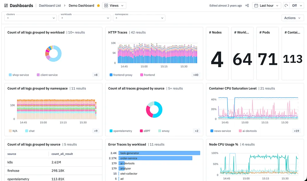


Monitoring request volume alone cannot tell you whether a service is healthy. Traffic may remain steady while requests start failing or response times increase. RED monitoring helps you detect these changes across services, giving you a consistent view of application performance and where problems need investigation.
This guide explains how to collect and query RED metrics using Prometheus and OpenTelemetry, build service dashboards, and configure SLO burn-rate alerts. It also covers how RED compares with USE and the four golden signals, how to apply it to different workloads, and how groundcover monitors these metrics.
What Is RED Monitoring?
RED monitoring measures the health and performance of request-driven services using three metrics: Rate (requests per second), Errors (failed requests), and Duration (request latency). Applying the same measurements across microservices helps you identify performance problems, compare service health, and investigate incidents consistently.
Rate: Requests per Second
Rate measures the number of requests a service handles per second. Track it across the entire service to understand overall demand, or by endpoint to see traffic changes on routes such as POST /checkout and GET /cart.
For example, a service might receive 400 requests per second during business hours and 40 overnight. Both can be normal, so compare request rates against their usual daily and weekly patterns. A sudden increase could indicate higher demand or repeated client retries, while a drop to zero during expected traffic might point to an upstream routing or availability problem. When requests never reach the service, its error count may remain unchanged.
Errors: Failed Requests and Error Ratios
Errors measure requests that fail. Track both the absolute error rate (failed requests per second) and the error ratio (failed requests divided by total requests). For example, two failures per second out of 400 requests per second produce a 0.5% error ratio. The same two failures out of four requests per second produce a 50% error ratio.
The error ratio lets you compare failure levels as traffic changes, while the absolute count shows how many requests are affected. For HTTP servers, 5xx responses generally indicate service failures. For HTTP server spans, 4xx responses normally leave the OpenTelemetry span status unset, although an unexpected 404 after a deployment can still indicate a broken endpoint.
Status codes do not capture every failure. A request can return HTTP 200 with incorrect content, time out before receiving a response, or exceed a committed response-time limit. Define which outcomes count as failures for each service level indicator (SLI). A 5xx-only error ratio cannot capture every availability failure, while slow but successful requests may violate a separate latency SLO.
Duration: Measuring Request Latency
Duration measures how long a request takes to complete. Track latency using percentiles such as p50, p95, and p99 because averages can hide slow requests.
Suppose 95 out of 100 requests complete in 50 ms while five take 2 seconds. The average latency is 147.5 ms, even though no request takes that long. Using the nearest-rank percentile method, p50 and p95 are 50 ms, while p99 is 2 seconds. The higher percentile reveals the slow requests that the average obscures.
Record request durations in histograms so you can aggregate latency measurements across service instances. Histograms count observations within duration buckets, allowing you to combine bucket counts from multiple pods before calculating percentiles. Averaging the p99 values calculated independently for each pod does not produce a valid service-wide p99.
Measure latency separately for successful and failed requests. An HTTP 500 returned immediately after a database connection failure can lower the overall latency measurement during an outage, making the service appear faster. Slow failures matter too, so retain error latency rather than excluding failed requests from the analysis.
RED vs. USE vs. the Four Golden Signals
RED measures request performance through rate, errors, and duration. Google’s four golden signals cover the same measurements as traffic, errors, and latency, with saturation as the fourth signal. Saturation reflects how close a service is to its capacity limits, including resource pressure that may affect performance before requests begin failing.
Brendan Gregg’s USE method focuses on the resources supporting a service rather than the requests it handles. It measures utilization (how busy a resource is), saturation (work waiting for a resource), and errors (resource-level failures). Its scope includes CPU, memory, storage, and network resources.
For example, a service’s p99 latency rises from 200 ms to 2 seconds. RED captures the slowdown, while USE metrics show whether CPU contention or disk saturation occurred during the same period. These resource measurements can narrow the investigation, although a matching spike does not necessarily mean resource pressure caused the slowdown.
Implementing RED Metrics With Prometheus and OpenTelemetry
To implement RED monitoring, you need request counts, error information, and latency measurements from your services. OpenTelemetry can collect these measurements, while Prometheus stores the resulting metrics and provides PromQL for calculating request rates, error ratios, and latency percentiles.
This walkthrough uses a Python Flask application to demonstrate the process. You’ll instrument the application, export its metrics to Prometheus over OTLP/HTTP, verify that the measurements are being collected, and query the three RED signals. You’ll need Python 3, Docker, curl, and a Bash-compatible terminal, with ports 8000 and 9090 available.
Instrumenting Services for RED Metrics
We’ll use an order endpoint that returns HTTP 200 for successful requests and HTTP 503 for a test failure. Having both responses makes it possible to verify request counts, error ratios, and latency measurements against known application behavior.
Create a file named app.py:
OpenTelemetry can instrument Flask automatically, so there’s no need to add metric-recording code to each request handler. Create a Python environment and install the required packages:
The bootstrap command detects supported libraries in the environment and installs their instrumentation packages, including the Flask instrumentation.
For HTTP servers, OpenTelemetry uses the http.server.request.duration histogram to record request durations in seconds. Each observation contributes to the histogram’s request count, while attributes describe the request and its outcome.
The attributes relevant to RED monitoring include:
http.request.method: Identifies the HTTP method, such asGETorPOST. Unknown methods are recorded as_OTHER.http.response.status_code: Records the response status when available, allowing HTTP 5xx failures to be counted separately.http.route: Identifies the matched route template, such as/orders/<int:order_id>, when the framework provides it.error.type: Identifies failed operations, including failures that occur before an HTTP response is available.
The histogram’s count provides Rate, status-code or error attributes identify Errors, and duration buckets provide the measurements needed to calculate latency percentiles.
Route labels should identify endpoint templates rather than individual URLs. Requests to /orders/123 and /orders/456 should belong to the same route series. Recording order IDs, user IDs, or request IDs as metric attributes creates unnecessary time series and increases monitoring costs.
Sending OpenTelemetry Metrics to Prometheus
Prometheus normally collects metrics by scraping HTTP endpoints, but it can also receive OpenTelemetry metrics directly through OTLP/HTTP. For this example, the Flask application will export its measurements to Prometheus without an intermediate Collector.
Create a rules directory to hold Prometheus alerting rules:
In the same directory as app.py, create a file named prometheus.yml with the following configuration:
Start Prometheus in Docker with the OTLP receiver enabled and both the configuration file and rules directory mounted:
Prometheus will be accessible at http://localhost:9090, with OTLP metrics ingestion available at /api/v1/otlp/v1/metrics.
The command uses the current Prometheus container image rather than requiring a particular release. For production deployments, pin a version you’ve tested. The OTLP receiver must be supported by the version you use, and it should not be exposed to untrusted networks because it has no built-in authentication.
Leave Prometheus running and open another terminal in the directory containing app.py. Activate the Python environment and configure the OpenTelemetry exporter:
The application now records HTTP request metrics and exports them every 15 seconds. The checkout service name becomes the job label in Prometheus, allowing you to query its measurements independently of other services.
The metrics-specific endpoint includes the complete /v1/metrics path. When OTEL_EXPORTER_OTLP_METRICS_ENDPOINT is configured, OpenTelemetry uses the URL as written rather than appending the path automatically.
The OTEL_SEMCONV_STABILITY_OPT_IN=http setting selects stable HTTP semantic conventions in instrumentations that support this option. Older instrumentation can still emit http.server.duration in milliseconds instead of http.server.request.duration in seconds. Confirm the metric name produced by your application before relying on the example queries.
In Kubernetes or other multi-service environments, an OpenTelemetry Collector can receive metrics from several applications and forward them to Prometheus. It also supports batching, filtering, and resource enrichment. The direct connection used here is sufficient for a local implementation.
Verifying That RED Metrics Are Being Collected
With Prometheus and Flask running, open a third terminal and send two requests:
The first should return HTTP 200 and the second HTTP 503. Both requests contribute to the request count and latency histogram, while the 503 response contributes to the HTTP 5xx error count.
Generate additional requests to establish a measurable request rate:
The loop sends 100 requests over approximately 50 seconds, with every tenth request returning HTTP 503. During the test, the error ratio should approach 10%.
Open the Prometheus expression browser at http://localhost:9090 and run:
After the application has exported its measurements, the query should return the request counts, separated by attributes such as http_response_status_code.
With Prometheus’s default OTLP translation strategy, http.server.request.duration becomes http_server_request_duration_seconds. Its classic histogram representation provides three related series:
http_server_request_duration_seconds_count: The total number of recorded requests.http_server_request_duration_seconds_bucket: Cumulative request counts within each duration boundary.http_server_request_duration_seconds_sum: The total recorded request duration in seconds.
These series provide the measurements for calculating all three RED signals.
If the count metric does not appear, check whether the application received requests, whether the exporter can reach Prometheus, and whether the OTLP receiver is enabled. Also check the emitted metric name, since instrumentation and translation settings can affect naming.
A raw request counter can appear after the first export, but rate() requires multiple samples. The generated traffic and 15-second export interval provide enough samples for the following queries.
PromQL Queries for Rate, Error Ratio, and p99 Duration
The following queries calculate RED metrics over five-minute windows using the classic histogram from the preceding setup. They aggregate by job, so requests from multiple instances of the same service contribute to a single result.
Request rate: Requests per second
The histogram’s _count series increases as requests complete. rate() calculates the average number of requests per second over five minutes, and sum by (job) combines measurements from all service instances.
Calculate rate() before summing the counters. If an instance restarts, its counter resets to zero, and Prometheus needs to account for that reset before aggregating across instances.
For the Flask example, the query should show a nonzero request rate while the test traffic is being recorded.
Error ratio: Failed requests as a percentage of traffic
The numerator counts requests returning HTTP 5xx responses, while the denominator counts all recorded HTTP requests. The or on (job) fallback returns zero when a service has traffic but no recorded 5xx errors, preventing an empty error-ratio result. Monitor missing traffic separately.
For example, an error ratio of 0.005 means 0.5% of requests failed. In the Flask test, the ratio should approach 0.1, or 10%, because every tenth generated request returns HTTP 503.
This query measures HTTP 5xx failures, not every application failure. A request might fail before returning a response or return HTTP 200 with incorrect content. Additional application-specific measurements may be necessary, depending on how you define successful requests in your SLI.
Duration: p99 request latency
The histogram’s _bucket series records how many requests completed within each duration boundary. histogram_quantile() uses the aggregated buckets to estimate the 99th-percentile latency.
The le label identifies the bucket boundaries and must remain in the aggregation. The result is measured in seconds, so a value of 0.35 represents an estimated p99 latency of 350 milliseconds.
The result is also an estimate rather than an exact percentile. Its accuracy depends on the histogram boundaries, particularly the width of the bucket containing p99. Choose boundaries close to the response-time thresholds that matter to your application.
For endpoint-level monitoring, include http_route in the aggregation:
You can also add http_route to the request-rate query and both sides of the error-ratio query. Endpoint-level measurements reveal failures or latency increases that might be difficult to distinguish in service-wide metrics.
These queries assume classic Prometheus histograms. If your setup stores native histograms instead, the latency query uses the base metric name without the le label:
For native histogram request counts, use histogram_count() rather than a separate _count series.
The default OTLP configuration used in this walkthrough produces classic histograms, so the earlier queries are appropriate. Before adding them to dashboards and alerts, confirm the actual metric names, labels, and histogram format in your Prometheus instance.
With request rates, error ratios, and latency percentiles available, you have the three measurements needed to build RED dashboards and define availability and latency SLOs.
Building RED Dashboards and SLO Alerts
Once you’ve collected RED metrics, you can use them to monitor service performance and alert on reliability problems. Dashboards show how request rates, failures, and latency change over time. SLO alerts notify you when those failures threaten your service’s reliability targets.
Designing a RED Dashboard per Service and Endpoint
A RED dashboard needs three main panels, using the PromQL queries from the previous section:
- Request rate: Requests per second, showing changes in traffic and unexpected drops.
- Errors: Failed requests per second and the error ratio, with their units clearly distinguished.
- Duration: p50, p95, and p99 request latency, showing both typical response times and slower requests.
In Grafana, create dashboard variables for job and http_route so you can switch between services and endpoints without duplicating dashboards. Use a consistent query window, such as five minutes, across the panels.
Display the error ratio as a percentage and latency in milliseconds. For the latency panel, use the histogram_quantile() query from the previous section with 0.50, 0.95, and 0.99 to plot the three percentiles.
Endpoint-level views are important because service-wide measurements can conceal failures on less frequently used routes. A checkout endpoint might fail completely while the overall error ratio remains low because other endpoints continue handling requests successfully.
Mapping RED Metrics to SLOs and Alerts
RED metrics can provide the service level indicators (SLIs) used to measure availability and latency against service level objectives (SLOs).
For example, a service could have these 30-day objectives:
- Availability SLO: 99.9% of recorded requests succeed, allowing a 0.1% error budget.
- Latency SLO: 95% of recorded requests complete within 500 ms, allowing 5% to exceed that threshold.
The availability SLI uses the error ratio calculated earlier. For latency, the proportion of requests completing within 500 ms can be measured using the duration histogram:
This query measures the five-minute latency SLI. The le="0.5" bucket must exist in your histogram; check the actual bucket boundaries before using it. Evaluating compliance with a 30-day SLO requires measurements covering the full 30-day period.
Rather than paging whenever an error ratio crosses a fixed threshold, use SLO burn-rate alerts. Burn rate measures how quickly failures consume the allowed error budget. A burn rate of 1 means the service is consuming its budget at exactly the rate permitted by its SLO.
For a 99.9% availability SLO over 30 days, these are useful starting points:
Each alert checks both windows. The longer window establishes that the service has experienced significant failures, while the shorter one confirms that the problem is still occurring.
For the 14.4× alert, the error ratio must exceed 1.44% over both one hour and five minutes. Create a Prometheus rule file named red-alerts.yml:
Save the alerting rule as rules/red-alerts.yml in the directory containing prometheus.yml. The rules directory is already mounted inside the Prometheus container, so you can validate the file without installing Prometheus locally.
Open another terminal and run:
If validation succeeds, restart Prometheus to load the rule:
Open http://localhost:9090/alerts and confirm that CheckoutAvailabilityBurn appears. Prometheus evaluates the alert against the configured error-ratio thresholds.
Prometheus evaluates the rule, but sending notifications requires an Alertmanager configuration. Alertmanager handles notification routing, grouping, and silencing.
The same burn-rate approach applies to latency SLOs, using requests that exceed the latency target as bad events and the latency SLO’s allowed failure fraction as the budget. Additional rules can cover the slower burn rates in the table.
Request-rate changes alone generally do not justify paging. A service can also stop receiving traffic without recording errors, so unexpected traffic loss needs a separate availability or synthetic monitoring check. Low-traffic services need particular care because a single failed request can produce a large error ratio.
Applying RED to gRPC, Queues, Databases, and Batch Jobs
RED monitoring also works for services that don’t handle HTTP requests. The main difference is what counts as a request: a gRPC call, a processed message, a database operation, or a job execution. Each workload needs a clear definition of successful and failed operations.
- gRPC: Measure calls per second, failed calls, and call duration. OpenTelemetry’s
rpc.server.call.durationhistogram measures incoming calls in seconds, withrpc.status_codeidentifying the result. For server-side calls,UNKNOWN,DEADLINE_EXCEEDED,UNIMPLEMENTED,INTERNAL,UNAVAILABLE, andDATA_LOSSgenerally count as errors, while client-side calls generally treat all non-OKstatuses as errors. Define failures according to your SLI and the operation’s expected outcomes. - Queue consumers: Measure successfully and unsuccessfully processed messages per second, processing failures, and processing duration. OpenTelemetry’s
messaging.process.durationmeasures processing time, whileerror.typeidentifies failures. Don’t confuse messages delivered to a consumer with messages processed successfully. Themessaging.client.consumed.messagescounter measures deliveries, not completed processing. - Databases: Measure operations per second, failed operations, and query latency. Client instrumentation can use
db.client.operation.durationto track operation duration. Use error attributes to separate failed queries and group measurements by operation rather than individual SQL statements containing dynamic values. - Batch jobs: Measure completed runs per hour or day, failed runs, and execution duration. Because jobs run periodically, their RED metrics may be sparse between executions.
- Serverless functions: Treat each invocation as a request. Monitor invocation rate, failed invocations, and execution duration, including timeouts.
RED cannot detect work that never starts. A Kafka consumer that stops processing messages might record no new failures while its backlog grows. Monitor consumer lag using Kafka’s records-lag-max or kafka_consumergroup_lag when using Kafka Exporter. For Amazon SQS, ApproximateAgeOfOldestMessage measures the age of the oldest unprocessed message, subject to SQS’s handling of repeatedly failed messages.
Scheduled jobs need a similar check. In Kubernetes, compare kube_cronjob_status_last_successful_time against the expected execution schedule and alert when a successful run is overdue. Also account for jobs that have never succeeded, since they may have no last-success timestamp.
Keep resource utilization and saturation metrics alongside RED for troubleshooting. RED identifies changes in workload performance, while resource metrics help investigate CPU, memory, disk, or network contention.
Monitoring RED Metrics With groundcover
groundcover automatically collects RED metrics from Kubernetes workloads using its eBPF sensor, without requiring application code changes or per-service instrumentation. The sensor runs as a DaemonSet, capturing traffic from supported protocols such as HTTP, gRPC, PostgreSQL, MySQL, Redis, and Kafka. It associates requests with their workloads, namespaces, and pods, then calculates request rates, errors, and latency percentiles. This eBPF auto-instrumentation approach also captures traffic from newly deployed services as they begin handling requests.
Viewing RED Metrics and Investigating Failures
To monitor a service, open groundcover’s Explore page and select the APM data source. Use the available filters to narrow your measurements:
- Source: Select eBPF to examine automatically captured application traffic.
- Direction: Choose Inbound for requests your service handles or Outbound for requests it makes to dependencies.
- Resource type and endpoint: Narrow the view to a protocol, service, or API endpoint.
You can examine Request Rate, Errors, Error Rate, and AVG, P50, P95, or P99 Latency. Group measurements by labels such as namespace, workload_name, clustered_path, and response_status_code to compare services and endpoints. If the checkout service’s error rate increases, filter the measurements to the affected endpoint and response statuses, then inspect traces, application logs, and Kubernetes events to identify the affected workload and its dependencies.
For latency regressions, start with the affected service’s response-time percentiles, identify the slower endpoint, and inspect its traces to find the downstream operation causing delays. You can also use APM tracing to follow requests across services and isolate slow or failing operations.
Combining eBPF Metrics With OpenTelemetry
groundcover also accepts OpenTelemetry telemetry over OTLP, allowing you to retain existing instrumentation alongside automatic eBPF collection. OpenTelemetry spans can produce APM measurements for request counts, error rates, and latency, while the APM source picker lets you examine measurements from either collection method.
Custom OpenTelemetry metrics are available through groundcover’s Metrics data source, where you can use PromQL-compatible MetricsQL queries. Built-in RED measurements are available through the APM data source in Explore, dashboards, and monitors. By combining eBPF and OpenTelemetry, you can extend Kubernetes observability while retaining existing application instrumentation.
FAQs
Tom Wilkie developed the RED method while working at Weaveworks, drawing on Google’s Four Golden Signals, which he had used as a site reliability engineer at Google. He focused on Rate, Errors, and Duration to give teams a consistent way to monitor request-driven microservices. The method emphasizes service behavior rather than infrastructure resource utilization.
Yes. groundcover’s eBPF sensor automatically collects request rates, errors, and latency measurements from supported Kubernetes application traffic without requiring OpenTelemetry SDKs or application code changes. You can also ingest existing OpenTelemetry telemetry over OTLP and examine RED measurements through groundcover’s APM data source.
Not always. HTTP 4xx responses generally indicate client-side problems, but some can reveal application failures. For example, an unexpected 404 after a deployment may indicate a broken route. Define which status codes count as errors based on the endpoint’s expected behavior and your availability SLI.
Low request volumes make error ratios and latency percentiles sensitive to individual requests. Use longer evaluation windows or minimum request counts to reduce noisy alerts, and add synthetic checks to detect availability problems when real traffic is absent. Keep synthetic traffic separate from real-user SLIs unless your SLO explicitly includes it.
Not necessarily. A duration histogram’s _count series records the number of observed requests, while its buckets provide the latency distribution. With suitable status-code labels, the same histogram can support request rate, error ratio, and latency queries. Separate counters are useful when you need different labels or the histogram doesn’t cover every request.